Session 9: Approaches to Modeling

Part 2:
Approaches to Modeling

There are many different methods and approaches used in atmospheric modeling. Each style has its advantages and disadvantages. We will cover four styles of modeling: diagnostic, prognostic, Lagrangian, and Eulerian. These approaches are used for both meteorological and air quality models.

Diagnostic Models

When you go to the doctor, you might recieve a checkup. The doctor examines the information collected on your condition and then tells you other information about your condition based on the data collected. This is called a diagnosis.

In the same respect, a diagnostic model is one the takes certain data and simulates overall conditions for the atmosphere. For example, researchers receive data from radiosondes from around the nation. However, these radiosondes do not tell us everything about the atmosphere. So the data is put into a diagnostic model in order for us to extrapolate approximately what is happening throughout the atmosphere. From a small amout of initial data, we receive a large quantity of output data describing various processes occuring in the atmosphere at the time of observations and measurements. Diagnostic models tell you what's happening now, what the current conditions are.

Prognostic Models

If you were to go to the doctor with an injury or severe sickness, the doctor would examine you (give a diagnosis), and then tell you what would probably happen in the near future. For example, If you had pneumonia, the doctor might tell you that you could expect increased soreness and muscle stiffness, but that in two weeks you would feel better. This is called a prognosis.

Similarly, a prognostic model is one that takes initial data and gives a prediction about what the atmosphere will be like at some time in the future. The predictions that you see on the evening weather report is determined by using various prognostic models. Different models are used to predict different time steps. Some models are very accurate at 12 hour predictions. Others are more accurate at 48 hour predictions. Because different details and methods are used for each model, a good forecast meteorologist will look at several model outputs before making a prediction.

Lagrangian Models

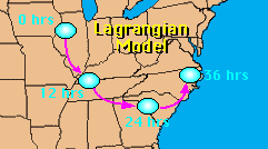
A Lagrangian model is simply one which uses the Lagrangian derivative, d/dt . This is simply the total change of any scalar with time. What does the total derivative mean? It means that in the model, the user is following a parcel of air as it travels through the atmosphere. The parcel is not set in any fixed location. A Lagrangian model simulates the movement of the air parcel and the changes that it undergoes because of that movement. Therefore, any changes to the parcel are due to the changes in the atmosphere through which the air parcel moves.

Eulerian Models

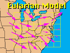
A Eulerian Model uses the Eulerian derivative,

. The Eulerian, or partial derivative, is the local change of any scalar with time. This is the opposite of the Lagrangian derivative. In a Eulerian model, the location is fixed, and the model simulates air movement in and out of the area of interest. A Eulerian model does not follow an air parcel, but focuses on a set location, which does not move. A Eulerian model usually uses a grid setup, in which the model outputs data for each grid cell (see Grids in Session 5). Because the location that the model simulates is permanent, the boundaries of the zone of interest are also permanent. It is therefore crucial to the model accuracy to make sure that the input data is appropriate and accurate at the boundaries of the model zone. If the initial information is corrupted or inaccurate, then any output data will also be grossly inaccurate. In order to continuously make sure that the boundary conditions are accurate, models use four-dimensional data assimilation (FDDA) to insert observed data into the grid boundaries at the appropriate time steps. We will discuss FDDA in Part 6 of this session.

On to Meteorological Models

Back to Introduction to Numerical Modeling

Developed by